Table of Contents
- Introduction to Huffman Coding
- How Huffman Coding Works
- The Problem with Naive Variable-Length Codes
- Why Huffman Trees Solve the Prefix Problem
- How the Tree Decides Code Lengths
- A Sample Frequency Table and Its Tree
- Building the Tree Step by Step
- Generating Huffman Codes from the Tree
- Encoding and Decoding Data Using Huffman Codes
- Canonical Huffman Coding
- Limitations of Huffman Coding
- Conclusion
Introduction to Huffman Coding
Huffman coding is one of the oldest and most widely used lossless compression algorithms. It was developed by David A. Huffman and published in 1952 in his paper "A Method for the Construction of Minimum-Redundancy Codes". Despite being more than seventy years old, the core idea behind it still shows up today inside formats like DEFLATE, JPEG, and MP3.
At its heart, Huffman coding is built around one simple observation: not every symbol in a piece of data appears with the same frequency, so it makes no sense to spend the same number of bits on all of them. Symbols that occur often should get short codes, and symbols that rarely occur can afford to get longer codes. That single idea is the intuition you need to carry through the rest of this article.
How Huffman Coding Works
To see why this matters, let's start from something familiar: fixed-length ASCII encoding. Every ASCII character is represented using exactly 8 bits, regardless of how often it appears in the text. Take the string "abcaaabcccaax" as an example. Encoded in plain ASCII, it looks like this:
01100001 01100010 01100011 01100001 01100001 01100001
01100010 01100011 01100011 01100011 01100001 01100001
01111000
That's 13 characters, each taking up 8 bits, for a total of 104 bits. But if we look closely at how often each character actually appears, we notice the distribution is far from even:
| Character | Frequency | ASCII Code |
|---|---|---|
| a | 6 | 01100001 |
| c | 4 | 01100011 |
| b | 2 | 01100010 |
| x | 1 | 01111000 |
The letter a alone makes up almost half the string, while x shows up only once. It clearly doesn't make sense for both of them to cost 8 bits. The character that appears the most, a, should be assigned the shortest possible code, and the character that appears the least, x, can be given the longest code. Over the length of the whole message, this trade-off pays off: the frequent characters save far more bits than the rare characters cost.
There's one detail we can't skip, though. If we're going to replace the standard ASCII table with our own custom, frequency-based table, the receiver has no way of knowing what that table looks like unless we tell them. So the dictionary itself, the mapping between characters and their new codes, has to be embedded in the encoded data (or otherwise agreed upon in advance), so the decoder knows how to translate the bits back into the original characters.
The Problem with Naive Variable-Length Codes
So let's try assigning shorter codes naively, based purely on frequency, and see what happens. Here is one possible table:
| Character | Frequency | Code |
|---|---|---|
| a | 6 | 0 |
| c | 4 | 1 |
| b | 2 | 01 |
| x | 1 | 11 |
At first glance this looks reasonable: the most frequent characters get the shortest codes. But this table hides a serious flaw. Suppose the receiver gets the following bit stream, encoded with this table:
0011Can you decode it? Try it for a moment before reading on. The honest answer is: you can't, at least not reliably, because there are multiple valid ways to split those four bits according to the table above:
0 01 100 110 0 110 0 1 1
All four groupings are technically valid under the table we built, yet they decode to completely different characters. The root cause is that some codes are prefixes of other codes: 0 is a prefix of 01, and 1 is a prefix of 11. As soon as one code can be the start of another, the decoder has no way to know where one symbol ends and the next one begins.
So we need a smarter way of assigning codes, one that respects frequency while guaranteeing that no code is ever a prefix of another code. That's exactly the problem the Huffman tree was built to solve.
Why Huffman Trees Solve the Prefix Problem
Before looking at an actual Huffman tree, it helps to be explicit about what we actually need from our code table. We want an assignment of codes to characters that satisfies two rules:
- Code length should depend on frequency: characters that occur often get short codes, and characters that occur rarely get longer codes.
- No code can be a prefix of another code, so the decoder is never left guessing where one symbol ends and the next begins.
A binary tree turns out to satisfy both rules naturally, as long as we follow one constraint: every character must live on a leaf node, never on an internal node.
Internal nodes aren't characters at all. They're just placeholders that represent "everything beneath me combined occurs this many times." The actual characters only exist at the leaves, and the code for a character is simply the sequence of left/right turns you take to walk from the root down to that leaf.
This is exactly what guarantees the no-prefix rule. Since a character only exists at a leaf, and a leaf by definition has no children, there is no way for another character's path to continue past it. If a code were a prefix of another code, that would mean the path to one character continues on to reach a second character, which would require the first character to sit on an internal node with a child beneath it. But we never allow that. Every character is a dead end. That's the entire guarantee, and it's why the Huffman tree structurally cannot produce ambiguous codes.
How the Tree Decides Code Lengths
So the leaf-only rule takes care of the ambiguity problem. But how does the tree decide how deep each character should sit, in other words, how does it enforce our first rule, that frequent characters get shorter codes?
The algorithm builds the tree from the bottom up, starting at the leaves and working toward the root. Think of each character's frequency as a weight. At every step, the algorithm looks at all the current items (characters or already-merged groups) and picks the two with the smallest weight. It ties those two together under a new parent node, and from now on treats that parent as a single combined item, whose weight is the sum of its two children.
Every time two items are merged this way, both of them gain one extra bit in their eventual code, because reaching either one now requires walking one extra edge down from their new shared parent. Since we always merge the two lightest items available, we are deliberately handing out that extra bit of length to the characters that occur the least. That's a cheap trade: penalizing a rare character by one extra bit barely affects the total size of the file, while doing the same to a frequent character would be expensive.
This process repeats over and over. Frequent, "heavy" characters tend to stay unmerged for a long time, since there are almost always lighter items available to merge first. That means heavy characters get pulled into the tree late, which keeps them close to the root and gives them a short path, and therefore a short code. Rare, "light" characters get merged early, get buried deeper in the tree, and end up with longer codes. This bottom-up, always-merge-the-two-lightest strategy is precisely what guarantees that code length ends up inversely related to frequency.
A Sample Frequency Table and Its Tree
To make this concrete, consider the following set of characters and frequencies:
| Character | Frequency |
|---|---|
| A | 16 |
| B | 5 |
| C | 12 |
| D | 17 |
| E | 10 |
| F | 25 |
Building a Huffman tree from this table, always merging the two lowest-frequency items, produces the tree shown below. By convention, we'll label every left branch 0 and every right branch 1:
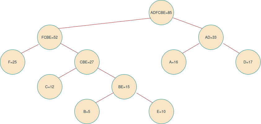
Reading the path from the root down to each leaf gives us the final code for every character:
| Character | Code | Frequency |
|---|---|---|
| F | 00 | 25 |
| D | 11 | 17 |
| A | 10 | 16 |
| C | 010 | 12 |
| E | 0111 | 10 |
| B | 0110 | 5 |
Notice what happened: F and D, the two most frequent characters, ended up with the shortest codes at just 2 bits each, while B, the least frequent character, ended up with a 4-bit code. None of the codes are a prefix of any other, exactly as our two rules required.
Building the Tree Step by Step
It's worth walking through exactly how that tree was assembled, one merge at a time, since the process itself is simple to repeat by hand.
Step 1 : Starting table
A: 16 B: 5 C: 12 D: 17 E: 10 F: 25Step 2 : Merge the two lowest: B (5) and E (10)
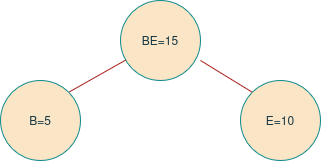
Updated table:
A: 16 C: 12 D: 17 F: 25 BE: 15Step 3 : Merge the two lowest: C (12) and BE (15)
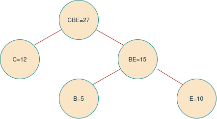
Updated table:
A: 16 D: 17 F: 25 CBE: 27Step 4 : Merge the two lowest: A (16) and D (17)
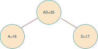
Updated table:
AD: 33 F: 25 CBE: 27Step 5 : Merge the two lowest: F (25) and CBE (27)
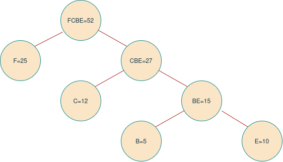
Updated table:
AD: 33 FCBE: 52Step 6 : Only two items remain: merge AD (33) and FCBE (52)
This final merge produces the root of the tree, with a combined weight of 85, matching the full tree shown in the previous section:
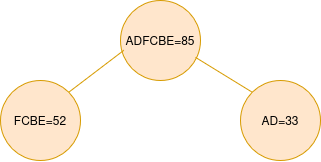
At this point there is nothing left to merge, so the tree is complete. Every character sits on a leaf, the two heaviest branches (AD and FCBE) hang directly off the root, and the lightest character, B, sits at the deepest point in the tree, exactly as the algorithm intends.
Generating Huffman Codes from the Tree
Once the tree is built, actually reading off the codes is the easy part. Starting from the root, every left branch you walk down contributes a 0 to the code, and every right branch contributes a 1. Keep walking until you land on a leaf, and the sequence of 0s and 1s you collected along the way is that character's code.
Do this for every leaf and you get the full code table, the same one we already built by hand in the previous section. Written as a small recursive procedure, the idea looks like this:
generate_codes(node, prefix):
    if node is a leaf:
        code_table[node.character] = prefix
        return
    generate_codes(node.left,  prefix + "0")
    generate_codes(node.right, prefix + "1")
Call this on the root with an empty prefix, and by the time it finishes, every character has a code that is guaranteed to be prefix-free, for exactly the reason we walked through earlier: it lives on a leaf, and leaves have no children for another code to continue into.
Encoding and Decoding Data Using Huffman Codes
Having a code table is one thing. Actually using it to encode and decode data is another, and this is where Huffman coding gets a little less convenient than plain ASCII.
With ordinary ASCII, every character is exactly 8 bits, so there's nothing to "decode" in the traditional sense. The CPU fetches one byte, and that byte is the character. Bytes and characters line up perfectly.
Huffman codes break that assumption. A code can be 2 bits, 3 bits, 7 bits, whatever the tree decided, and none of that lines up neatly with byte boundaries. So before we can write Huffman-encoded data to a file or send it over a network, we need a way to pack these odd-length codes together, bit by bit, into a continuous stream of bytes. That's the job of what we can call a bitstream: a small structure that lets us append an arbitrary number of bits at a time, in order, and read them back the same way.
Representing a single code
A single Huffman code needs two pieces of information, not one: the bit pattern itself, and how many bits long that pattern is. It's tempting to represent a code as just a number, but that breaks down immediately. The code 01 and the code 1 are both the number 1 if you drop the leading zero, yet they are two completely different codes. So a code is really a pair:
bitstream(value, length)where value is the bit pattern (it doesn't matter whether you write it in binary, hex, decimal, or octal, that's purely a matter of readability) and length is how many bits of that value actually count. The length field is what protects the leading zeros: bitstream(0b01, 2) and bitstream(0b1, 1) are both "the number 1" underneath, but the stream writes the first one as two bits and the second as one. You don't need a separate argument for "number of leading zeros", the length already tells you everything you need: pad the value on the left with zeros until it's exactly that many bits wide.
Encoding
Encoding a message, then, is just: for every character in the input, look up its (value, length) pair in the code table, and append those bits, in order, to the output stream. A minimal bit-writer that does this might look like:
typedef struct {
    uint8_t  current_byte;
    int      bits_filled;
    uint8_t *output;
} BitWriter;

void write_bits(BitWriter *bw, uint32_t value, int length) {
    for (int i = length - 1; i >= 0; i--) {
        int bit = (value >> i) & 1;
        bw->current_byte = (bw->current_byte << 1) | bit;
        bw->bits_filled++;

        if (bw->bits_filled == 8) {
            *bw->output++ = bw->current_byte;
            bw->current_byte = 0;
            bw->bits_filled  = 0;
        }
    }
}
Every call pushes one code's worth of bits into the buffer, flushing a full byte to the output every time 8 bits accumulate. Decoding runs the same idea in reverse: read one bit at a time from the stream, and use each bit to step either left or right from the root of the Huffman tree. The moment you land on a leaf, you've decoded one character, so you emit it, jump back to the root, and keep reading bits for the next character.
The problem of unaligned bytes
There's a catch, though. A message almost never encodes to a whole number of bytes. Suppose the encoded output comes out to 3 full bytes plus 3 extra bits. Those 3 leftover bits aren't enough to form a full byte on their own, but we still have to store or transmit them somehow, which means padding the last byte out to 8 bits.
That padding creates a real problem: the decoder has no built-in way to know where your actual data ends and the padding begins. If it keeps reading past the real message, those extra padding bits will get interpreted as the start of another code, and depending on the tree, that can silently produce a phantom extra character (or several) that was never part of the original message.
There are two common, and equally valid, ways to fix this:
- Store the exact bit count (or character count) alongside the data. A small header field before the compressed payload tells the decoder precisely how many bits (or how many characters) are meaningful. Once it reaches that count, it stops, no matter what bits happen to follow.
- Reserve a dedicated end-of-stream symbol in the alphabet. Instead of tracking a count, you add one extra "character" to your Huffman tree that means "stop here," and encode it once at the very end of the message. The decoder simply decodes until it hits that special symbol. This is the approach DEFLATE itself uses, with a reserved end-of-block code in its symbol alphabet.
Either approach works. The count-based header is simpler to reason about; the end-of-stream symbol avoids needing a separate header field at all, at the cost of one extra entry in your tree. What you should never do is assume the decoder can somehow "figure out" where padding starts, because from the bits alone, it can't.
Canonical Huffman Coding
So far we've assumed the decoder somehow already has the full tree, or at least the full code table, before it can decode anything. In practice, shipping the entire tree structure alongside the compressed data would eat into the savings we just worked so hard to get. This is where canonical Huffman coding comes in: a trick that lets us throw away the tree entirely and still reconstruct the exact same codes on the other side.
The key insight is that the actual bit patterns of a Huffman code don't matter for compression, only the code lengths do. Two different trees built from the same frequencies can assign completely different 0/1 patterns to the same characters and still compress to exactly the same number of bits, as long as every character ends up with the same code length in both trees. That means we don't need to transmit the tree, or even the specific bit patterns. We only need to transmit, for each character, how many bits its code should be. From that alone, both sides can independently derive the identical set of codes, as long as they follow the same rule for turning lengths into codes.
The canonical construction rule is simple:
- Sort the characters by code length (shortest first), and break ties alphabetically, or by whatever consistent ordering both sides agree on.
- Assign the first code, for the shortest length in the list, as all zeros.
- For every next character at the same length, add 1 to the previous code.
- Whenever the length increases, add 1 to the previous code first, then shift the result left by however many bits the length grew by.
Let's apply this to the same six characters we used earlier, where we already know each character's code length from the original tree: F and D and A at 2 bits, C at 3 bits, and B and E at 4 bits. Sorted by length, then alphabetically:
A: 2 D: 2 F: 2 C: 3 B: 4 E: 4Walking through the rule:
A (len 2): 00
D (len 2): 01              (previous + 1)
F (len 2): 10              (previous + 1)
C (len 3): 110             (previous + 1, then shift left by 1)
B (len 4): 1110            (previous + 1, then shift left by 1)
E (len 4): 1111            (previous + 1)
Notice that the bit patterns here are different from the ones we got out of the original tree (F was 00 there, and here it's 10), but every character has the exact same code length as before, which means the compressed size doesn't change at all. What we gained is that the receiver never needs the tree shape or the explicit codes. All we have to send is a compact list of lengths, something like A:2, D:2, F:2, C:3, B:4, E:4, and the decoder can regenerate this entire table on its own by applying the same four rules. That's a dramatic reduction compared to describing an entire binary tree, and it's exactly how real-world formats like DEFLATE store their Huffman tables.
Limitations of Huffman Coding
Huffman coding is elegant and cheap to run, but it isn't the last word in compression, and it's worth being upfront about where it falls short.
- Codes must be a whole number of bits. Huffman can never assign a character a code shorter than 1 bit, even if that character makes up 99% of the data. Information theory says such a character should ideally cost a small fraction of a bit, but Huffman has no way to express that. This is the main reason arithmetic coding and range coding can squeeze out extra savings that Huffman structurally can't reach.
- It needs the frequency table up front. The classic version of the algorithm requires scanning the entire input once to count frequencies before it can build a tree and start encoding. That's an extra pass over the data, and it means the encoder can't start emitting bits until it has already seen everything. (Adaptive variants of Huffman coding exist that update the tree on the fly, but they add their own complexity.)
- Small or skewed inputs suffer from overhead. Even in the canonical form, you still need to transmit a table of code lengths. For a short message, that overhead can outweigh the savings from shorter codes entirely, so Huffman coding tends to shine on larger inputs with a clearly uneven character distribution, not tiny ones.
- It only exploits frequency, not repetition. Huffman coding looks purely at how often each symbol occurs. It has no concept of repeated sequences or patterns, like the same word or byte pattern showing up over and over. That's exactly why real compressors don't rely on Huffman coding alone: formats like DEFLATE run a separate pass first (LZ77-style matching) to squeeze out repeated sequences, and only then hand the leftover symbols to a Huffman stage to shrink them further.
Conclusion
Looking back at everything we've covered, the whole idea behind Huffman coding really comes down to one trade-off, done well: spend fewer bits on the things that show up often, and don't worry about spending more on the things that barely show up at all. Everything else in this article, the leaf-only rule that kills ambiguity, the bottom-up merging that decides who gets the short codes, the bitstream tool that packs odd-length codes into real bytes, and the canonical form that lets us skip shipping the tree altogether, is really just the engineering needed to make that one idea work reliably in practice.
It's also worth remembering that Huffman coding isn't meant to be the whole compression story. On its own it only reacts to how often symbols appear, nothing more. That's precisely why it still shows up everywhere over seventy years later: not as a complete compressor by itself, but as the dependable final stage that squeezes real savings out of whatever symbols another algorithm hands it. Once you understand how the tree is built and how canonical codes are reconstructed from nothing but a list of lengths, you've understood the part of DEFLATE, PNG, JPEG, and a long list of other formats that rarely gets explained clearly, and that, more than any single trick, is what makes Huffman coding worth learning properly instead of just using as a black box.